Forecast Uncertainty Tracks Credit Risk Without Credit Labels: A Year of Temporal Fusion Transformers in Production Underwriting

Abstract

We describe a year of operating PRF-1, a Temporal Fusion Transformer (TFT) as the primary revenue forecaster inside an embedded small-business lending stack. PRF-1 takes twelve months of merchant payouts and emits a twelve-month forecast distribution. It was trained without any credit labels. By credit labels we mean the binary default flags, delinquency events, charge-offs, and aggregated repayment-outcome panels that risk models conventionally consume to learn the boundary between loss-making and performing merchant trajectories.

None of those signals were exposed to PRF-1 during training. Across two partner deployments and four geographies we observed three findings that, taken together, change how a forecaster should be integrated into an underwriting system. First, within the space of modern neural forecasters, loss-function selection moves model behavior further than architecture selection.

Second, a distributional output is necessary, not optional and the width of the model’s own forecast interval is empirically correlated with downstream deployed credit risk signal and hence repayment friction, even though no repayment signal is ever shown during training. Third, PRF-1’s attention weights are interpretable enough at the per-cohort level to serve as runtime diagnostics.

We report calibration to within 0.6 percentage points of nominal coverage on a held-out cohort, an 84% directional-accuracy upper bound at the twelve-month horizon, and a monotone relationship between origination-time downside dispersion and the deployed PD score, validated on our internal 18-month simulator cohort used for friction analysis.

1. Introduction

Embedded lending platforms underwrite small businesses from cash-flow data that is directly observable on the platform itself. Revenue forecasting sits upstream of nearly every downstream decision, be it offer size, term, pricing, or monitoring. The dominant class of production forecasters in this setting is the exponential smoothing (ETS) family [Hyndman et al., 2008], trained per-merchant on trailing payout histories. ETS is robust and interpretable, and it is close to optimal on dense recurring-revenue cohorts. It degrades on the short, intermittent, ramp-shaped, and seasonally heterogeneous histories that characterize small-business platforms. Modern neural sequence models take the opposite trade, a single global model is fit jointly across the merchant panel [Salinas et al., 2020; Montero-Manso & Hyndman, 2021], pooling structural patterns across series so that short, intermittent, ramp-shaped, and seasonally heterogeneous merchants can borrow strength from cohorts with similar trajectories rather than being fit on their own limited history alone. The cost is per-merchant interpretability and a small accuracy give-up on the easiest, densest series, the regime where ETS is already strong.

The forecasting failure modes that matter for credit are asymmetric. Over-forecasting produces repayment stress. Under-forecasting starves a growing merchant of capital. Neither is symmetric in cost. Classical accuracy metrics do not encode this asymmetry, and a forecaster trained to minimize symmetric error is not directly aligned with the underwriting objective.

In December 2024 we began testing neural sequence models as a replacement. In May 2025 we deployed a Temporal Fusion Transformer [Lim et al., 2021] model to production on our largest partner book, and have since extended it across four additional geographies and a second partner. This paper documents what changed across that year. The contributions are (i) a within-family architecture comparison showing that modern neural forecasters cluster tightly on per-merchant accuracy on this problem (ii) a loss-function study showing that the training objective is the dominant axis for shaping production behavior (iii) an analysis of TFT attention probes as runtime interpretability tools rather than post-hoc explanations (iv) empirical evidence that origination-time forecast uncertainty, specifically the width of the lower tail, is consistent with the deployed credit risk signal, despite the forecaster having no repayment supervision during training.

2. Problem Setup and Architecture

Task. For each merchant m at origination time t, given a payout history {y_m,t-L,..., y_m,t-1} of length L = 12 monthly periods, predict the distribution of cumulative payouts over the next H = 12 periods. The training set is a panel of several hundred thousand merchant-month observations across multiple geographies, sliced into rolling-origin train and out-of-time test windows.

Architecture. We use a Temporal Fusion Transformer following Lim et al. (2021). A representative production configuration has three RNN encoder layers with hidden dimension 256, four interpretable multi-head attention heads, a quantile head emitting nine quantiles between P₁₀ and P₉₀, and approximately 6.2M parameters. Inference is sub-100 ms per batch on a single GPU. Per-geography training channels are used in place of a single pooled model: pooling smoothes across structurally distinct revenue distributions and degraded per-merchant accuracy in early experiments.

Baselines. We compare against an ETS implementation in production through 2025 (per-merchant fit, automatic component selection) and a rolling six-month window-average baseline. Both are evaluated on the same train-test splits as the neural models.

Evaluation. All comparisons use temporal holdouts strictly later than the training window. Random splits leak future information and are not used. The protocol enforces temporal disjointness between train and test, but not merchant disjointness, a merchant with training observations through period T may have test observations at T+H. This is standard rolling-origin practice and controls leakage from future to past, but it does not control for the model recalling recurring merchant patterns from training. We discuss the corresponding overfit risk in section 9. Metrics are reported at H ∈ {3, 6, 12} months separately. We report per-merchant standardized RMSE, sMAPE, and scaled RMSE (RMSSE). For distributional models we additionally report empirical coverage at nominal quantiles.

3. Architecture Comparison

We trained TFT [Lim et al., 2021], TiDE [Das et al., 2023], N-HiTS [Challu et al., 2023], RMoK [Han et al., 2024], an LSTM-DeepAR variant [Salinas et al., 2020], and a six-month window-average baseline on the same monthly revenue panel. Table 1 summarizes the comparison qualitatively.

The neural families clustered within a few percentage points of one another on per-merchant standardized RMSE at every horizon tested. TFT and TiDE led at longer horizons. Across four within-TFT variants (changes to hidden size, attention heads, encoder depth, time encodings), per-merchant median standardized RMSE moved by under two percentage points. The window-average baseline was worse, but not by the margin intuition suggests, consistent with the findings of Zeng et al. (2023).

We selected TFT for two reasons beyond marginal accuracy. The variable-selection networks make multi-covariate extension well-defined for later iterations of the system. The attention components, discussed in Section 7, are directly inspectable as a function of encoder lag and forecast horizon. This is a property the alternatives do not share, and it became the load-bearing piece of how the model is monitored in production.

4. Loss Function Selection

Holding the TFT architecture fixed, we varied the training objective. The losses we evaluated were Huber and MAE (symmetric, point-forecasting); pinball loss at several quantile levels (asymmetric point-forecasting); a LinEx loss that exponentially penalizes over-prediction; and a multi-quantile loss (MQLoss) that emits nine quantiles in a single forward pass [Wen et al., 2017].

Two findings emerged. First, loss-function variation moved per-merchant error further than any within-TFT architecture change tested. Second, the loss that produced the lowest symmetric error (Huber) was not the loss that produced the best production model: Huber-trained variants fitted closely to the conditional mean and over-predicted on the tail of high-variance merchants where over-prediction is most expensive. An asymmetric loss (pinball at τ = 0.4) traded a small accuracy reduction for substantially fewer guardrail violations. The MQLoss variant produced a calibrated distributional output in a single pass and is the basis for the calibration and uncertainty results that follow.

The general statement is that the loss function encodes a posture toward credit decisions. In a credit setting, that posture is a policy choice, not a tuning parameter. Architecture choices within the TFT family did not encode it; the loss did.

5. Directional Accuracy Against the Classical Baseline

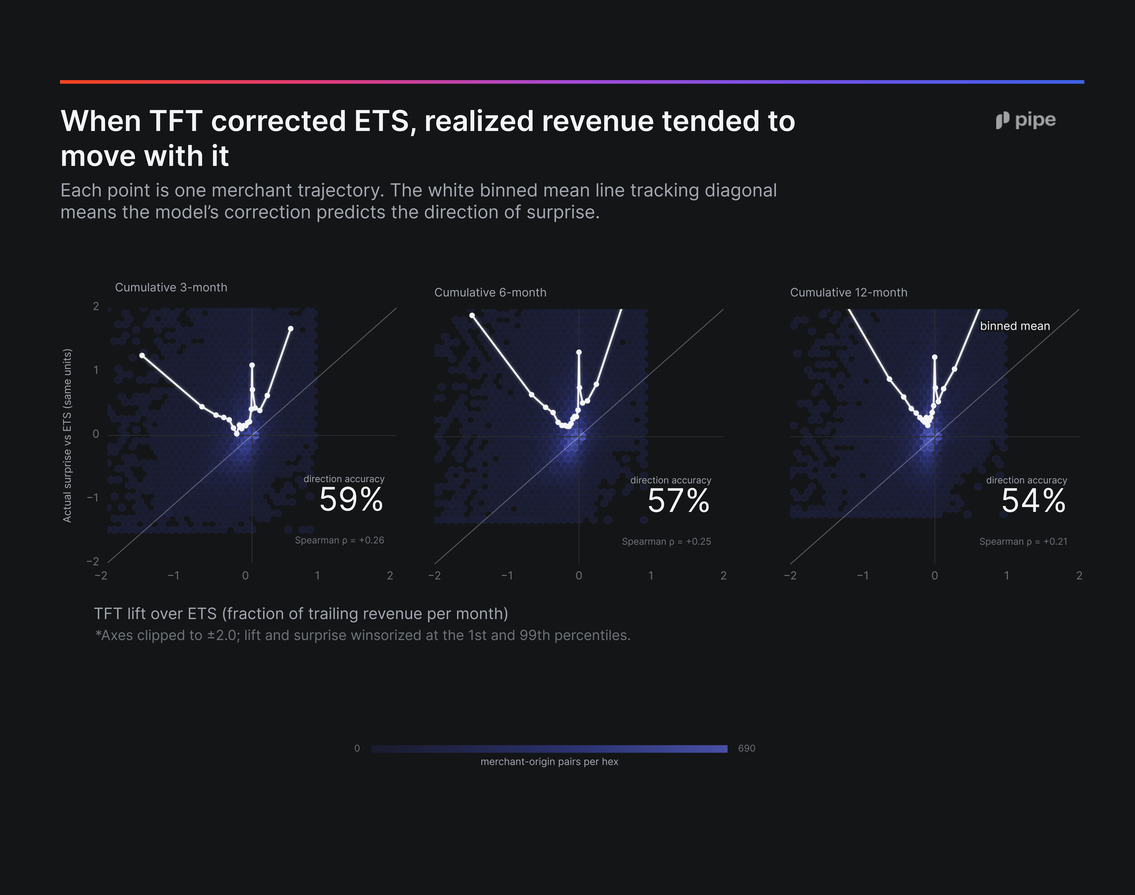
A useful test of whether a new forecaster recovers signal the prior system misses is to evaluate it against the prior system’s forecast rather than against truth alone. For each merchant-origin pair, we computed the PRF-1-minus-ETS difference at horizons H ∈ {3, 6, 12} months, normalized by trailing revenue, and measured whether the sign of that difference matched the sign of the realized surprise relative to the ETS forecast. Pairs with relative differences below 5 percent of trailing revenue were excluded as immaterial.

TFT vs ETS lift versus actual surprise

Figure 2: Cumulative TFT-minus-ETS lift (x-axis) against realized surprise relative to the ETS forecast (y-axis), at 3-, 6-, and 12-month horizons. Each point is one (merchant, origin) pair. The teal line is the binned mean of realized surprise across twenty quantile bins of the disagreement. Cells above the 45° dashed line are where TFT predicts the surprise direction correctly.

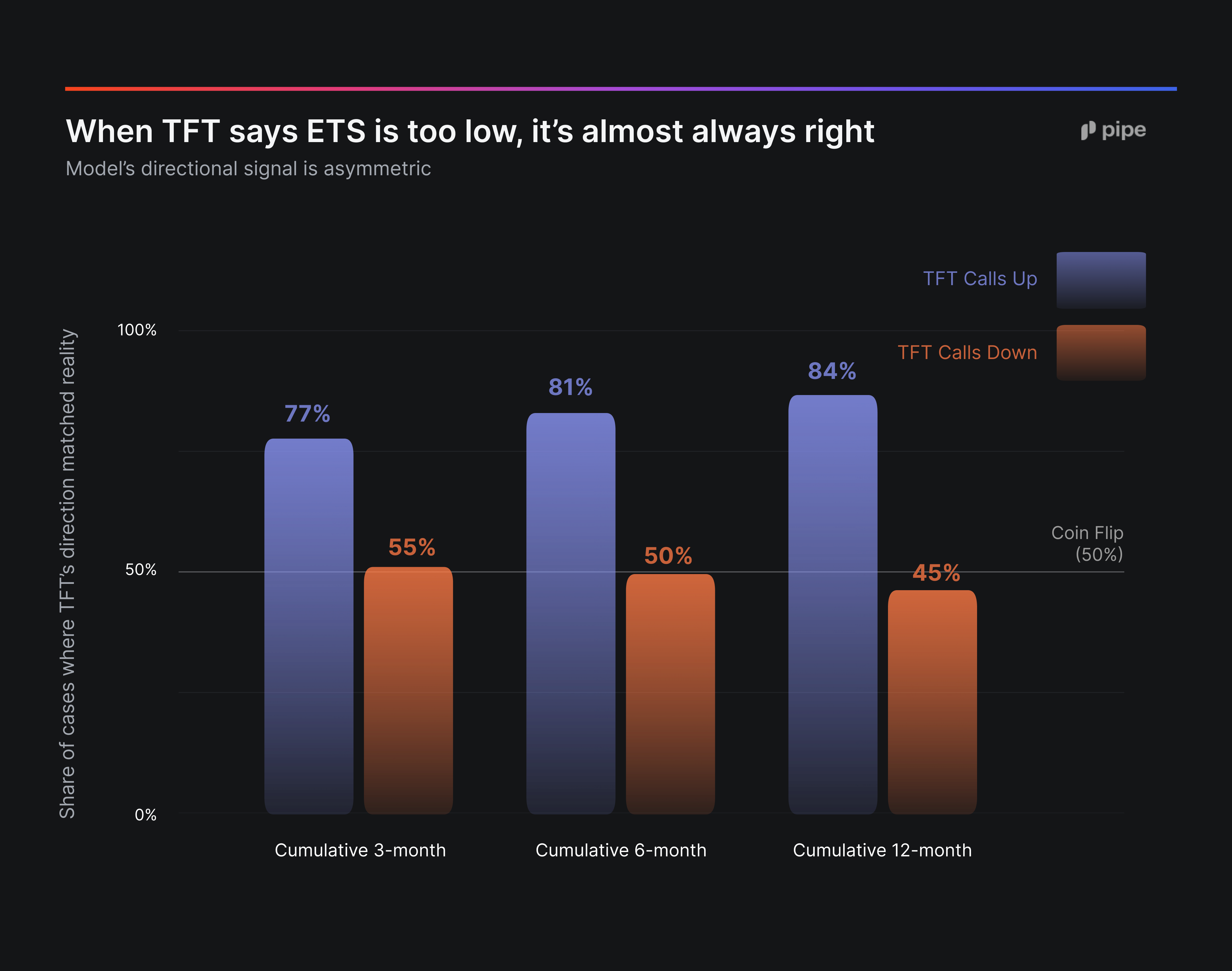
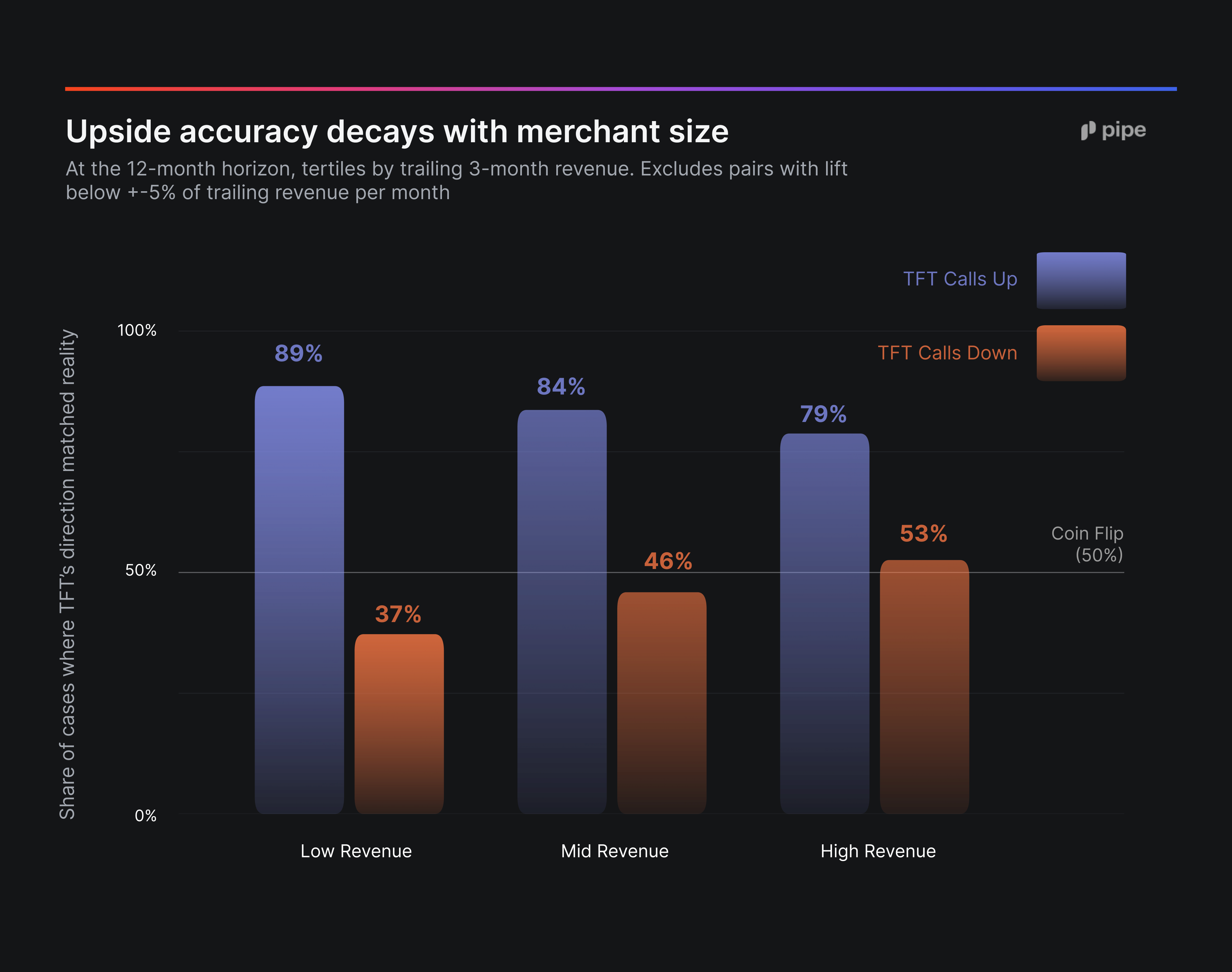
Among pairs where TFT predicted higher revenue than ETS, directional accuracy was 77 percent at three months, 81 percent at six months, and 84 percent at twelve months. Among pairs where TFT predicted lower revenue, directional accuracy was near coin-flip (55, 50, 45 percent respectively, n ~ 16,000 at each horizon). Stratifying by merchant size at the twelve-month horizon: upside directional accuracy was 89 percent on the smallest revenue tertile, 84 percent on the middle, and 79 percent on the largest. Downside accuracy did not improve with size.

Directional accuracy by horizon

Figure 3: For each horizon, the share of (merchant, origin) pairs where the model’s directional call against the ETS baseline matched the realized direction, split by whether the model disagreed upward or downward. Pairs with |lift| < 5% of trailing revenue are excluded.

Directional accuracy by merchant size

Figure 4: The same decomposition at the twelve-month horizon, stratified by trailing 3-month revenue tertile. The upward-correction signal is strongest on the smallest tertile, where the classical baseline has the least history to extrapolate from.

The asymmetry has a straightforward operational interpretation. The classical baseline is structurally cautious: it weights recent observations heavily and waits for evidence before extrapolating a trajectory.

The merchants on which TFT predicts higher revenue than the baseline are merchants whose recent trajectory has departed upward from the trailing average, and the TFT call is correct about that departure with high reliability. Where TFT predicts lower revenue, the call is not reliably correct: contraction signals are the job of risk models that consume behavioral, payment-history, and external inputs the revenue forecaster does not see.

We state this limitation plainly; the forecaster should not be used as the sole signal for contraction.

6. Forecast Distributions and Calibration

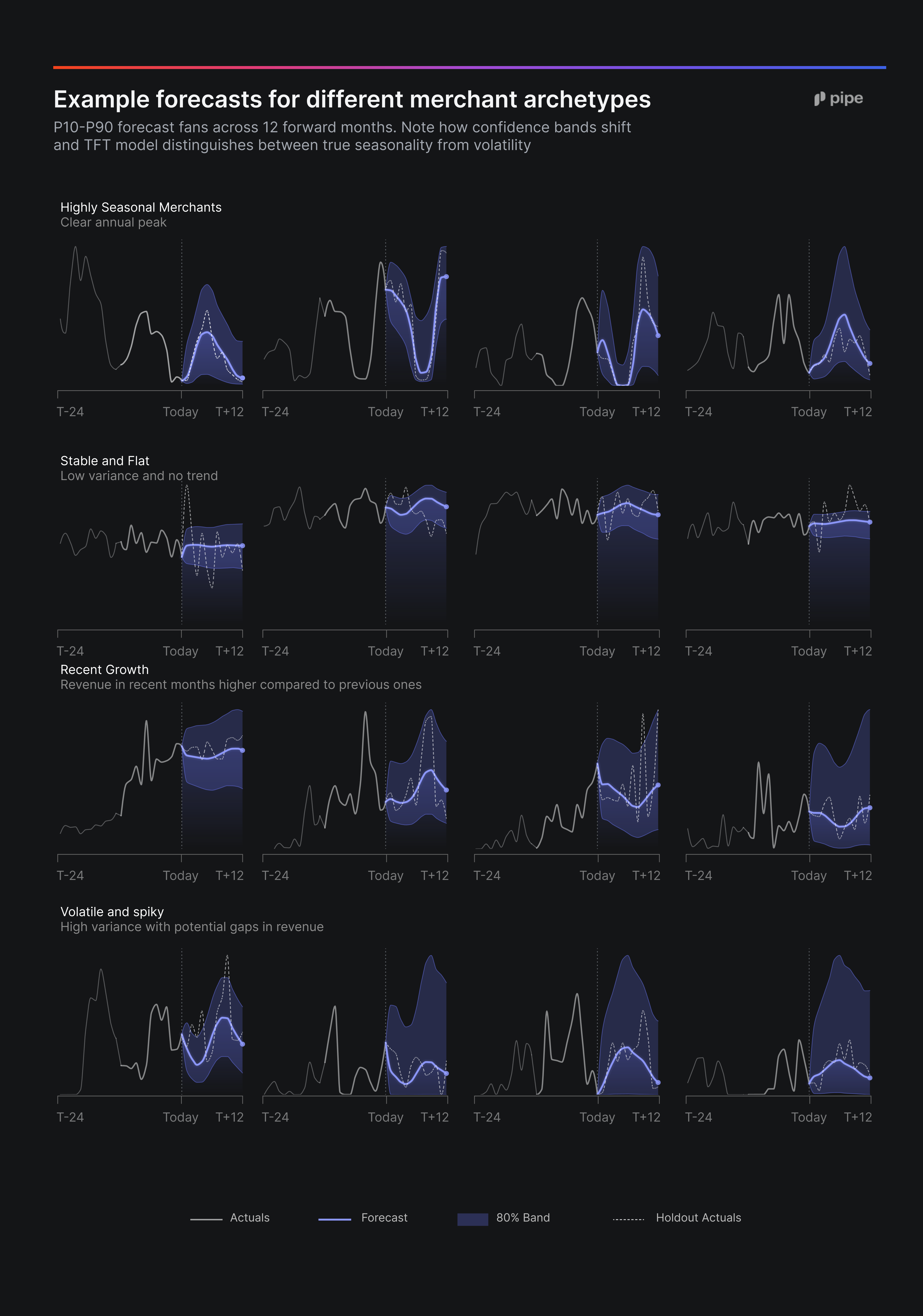
The MQLoss variant emits nine quantiles per forecast horizon. The width of the resulting interval is structurally different across merchant archetypes trained from the same model: highly seasonal merchants receive forecasts that themselves oscillate with narrow bands locked to the seasonal peak; stable merchants receive flat forecasts with narrow bands at the historical level; recently growing merchants receive moderate bands neither extrapolating exponential growth nor reverting to the long-run mean; volatile merchants receive bands spanning from near-zero to several multiples of the merchant’s average, paired with a median that tracks the broad trend without committing to any specific spike.

Same model, four merchant archetypes

Figure 5: Rows are merchant archetypes; columns are four exemplar merchants per archetype. The dark line is the merchant’s actual payout history. The green line and shaded band are the model’s median forecast and 80% prediction interval. The dashed line over the forecast region is the realized payout.

A calibrated quantile is a precondition for using a quantile as a policy variable. We evaluated empirical coverage against nominal quantile $\tau$ on a held-out backtest at the six-month horizon. On the subset of rows where the model emitted monotone quantiles, empirical coverage tracked nominal τ to within 0.6 percentage points across all nine quantiles. After a one-line cumulative-max post-processing step that re-imposes monotonicity on the remaining rows [Chernozhukov et al., 2010], coverage tracked nominal τ to within 2.2 percentage points across the full sample.

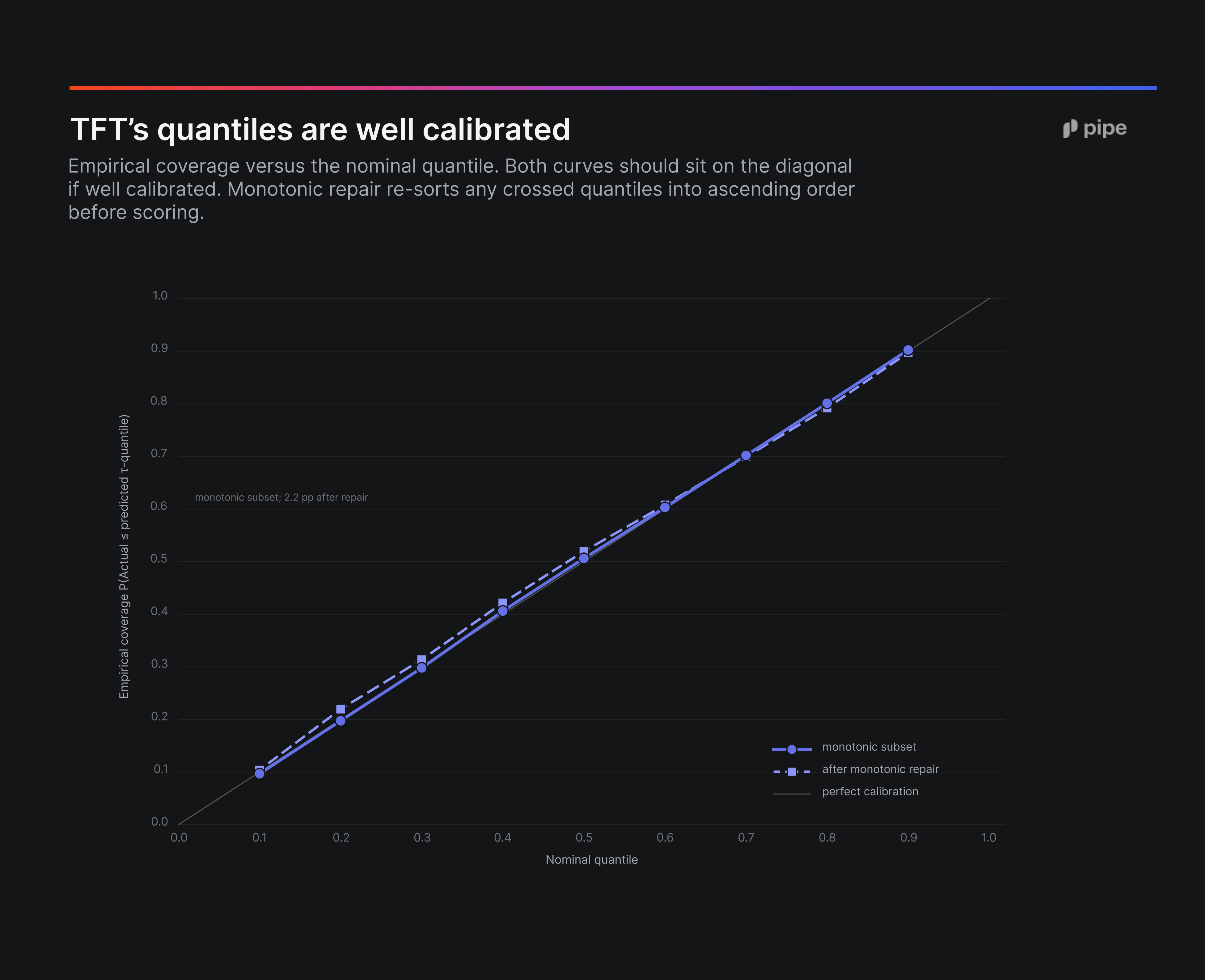Reliability diagram, 6-month horizon

Figure 6: Empirical coverage versus nominal quantile on the six-month horizon. The dark solid line uses the subset of forecasts where the model already emitted ordered quantiles. The lighter dashed line keeps the rows where the model emitted out-of-order quantiles and applies a one-line cumulative-max post-process.

Approximately 11 percent of otherwise-valid forecasts emitted at least one crossed quantile pair (a predicted P₂₀ exceeding the predicted P₃₀). This is a known artifact of training the nine quantile heads independently. Monotone rearrangement resolves it without distorting the calibration result and is applied unconditionally in the production pipeline.

The general point: a distribution that is statistically well-calibrated but structurally inconsistent is not consumable by a downstream policy layer. The model and the thin post-processing layer around it together produce the production signal; neither in isolation does.

7. Forecast Uncertainty as a Risk Signal

The model was trained on revenue alone, with no exposure to default flags, delinquency events, or repayment outcomes. We evaluated whether its output nevertheless carries credit-relevant information using an 18-month simulator backtest on a single-partner cohort of all merchants from one of our partners. At each simulator origin the TFT receives only the twelve monthly payouts strictly preceding that origin and emits a two pass -month forecast distribution; the encoder window and the forecast horizon are time-disjoint per-prediction, so no future revenue from a merchant's outcome window enters its own forecast. The simulator then replays the same merchant population through the underwriting policy twice: once with the TFT forecast as the input, once with the prior ETS forecast. Risk grade, collection mechanics, and the merchant's actual realized revenue stream are held constant across the two runs. As noted in Section 2 and discussed in Section 9, the rolling-origin protocol is temporally disjoint per-prediction but not merchant-disjoint across the panel: the model has seen these merchants at other origin slices during training, which we treat as an overfit-risk caveat rather than as evidence of leakage at scoring time. The outcome metric is repayment friction, measured as days past due at month 18 (DPD).

By merchant difficulty. Each merchant was assigned to a difficulty quartile by average friction across both runs (the bucketing is model-blind). Indexed friction reduction, relative to the population-average reduction set to 100: Q1 (easiest) 136, Q2 117, Q3 73, Q4 (hardest) 18. The TFT-driven policy reduced friction in every quartile, with the largest absolute reduction concentrated in the middle of the difficulty distribution, where there is enough friction for forecast quality to matter and enough predictability for the model to act on.

Against the deployed PD signal. A second view reads the forecaster's uncertainty against the production credit model directly. For each merchant we computed the relative downside gap (P_q - P₅₀) / P₅₀ at q ∈ {0.2 , 0.3} on the six-month horizon, then grouped merchants by their PD score from the deployed risk model. The downside gap widens monotonically as PD rises: at the P₂₀ tail it moves from approximately -0.30 in the lowest PD bin to approximately -0.70 in the highest; the P₃₀ tail traces the same shape, one band closer to the median. The pattern is stable across every PD bin with enough merchants to read cleanly.

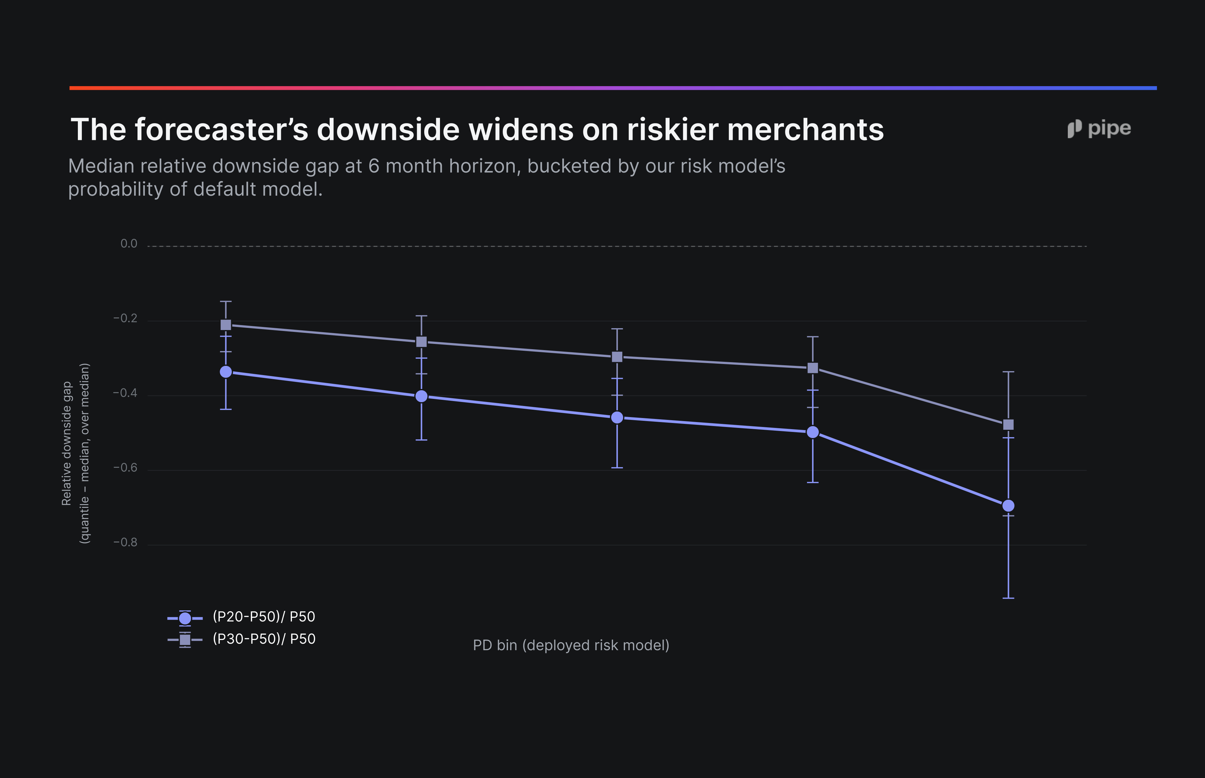The reading is that the same merchant heterogeneity that drives PD also drives the width of the TFT's lower tail. The unsupervised forecaster recovers a signal that the supervised PD model also recovers, convergent evidence on the same underlying structure, not an additional signal. A point-forecast system discards this dimension by construction.

We note the obvious limitation: this is a simulator result, not a randomized experiment. A prospective experiment in which sizing is keyed to model-emitted uncertainty is the natural next test.

8. Interpretation: What Attention Heads Learn

A practical advantage of the TFT family is that attention weights are directly inspectable as a function of encoder lag and forecast horizon. We extracted per-sample weights on a production cohort of merchants using a forward hook on the trained model (the published TFT API exposes only weights collapsed over batch and heads, which discards exactly the structure we wanted to study).

Per-head specialization. The four heads in the production model learned structurally distinct roles, with no supervision specifying what those roles should be:

• Head 0 concentrates approximately 35 percent of its weight on the oldest encoder position, invariant across forecast horizons. It anchors on long-run level.

• Head 1 shifts along a near-perfect diagonal as the forecast horizon advances: correlation between forecast step and peak-weight encoder position is approximately 0.99. This is the seasonality probe.

• Head 2 concentrates on a fixed mid-range position (approximately nine periods back) plus the most recent observation, reused across horizons.

• Head 3 distributes attention broadly and is residual in character.

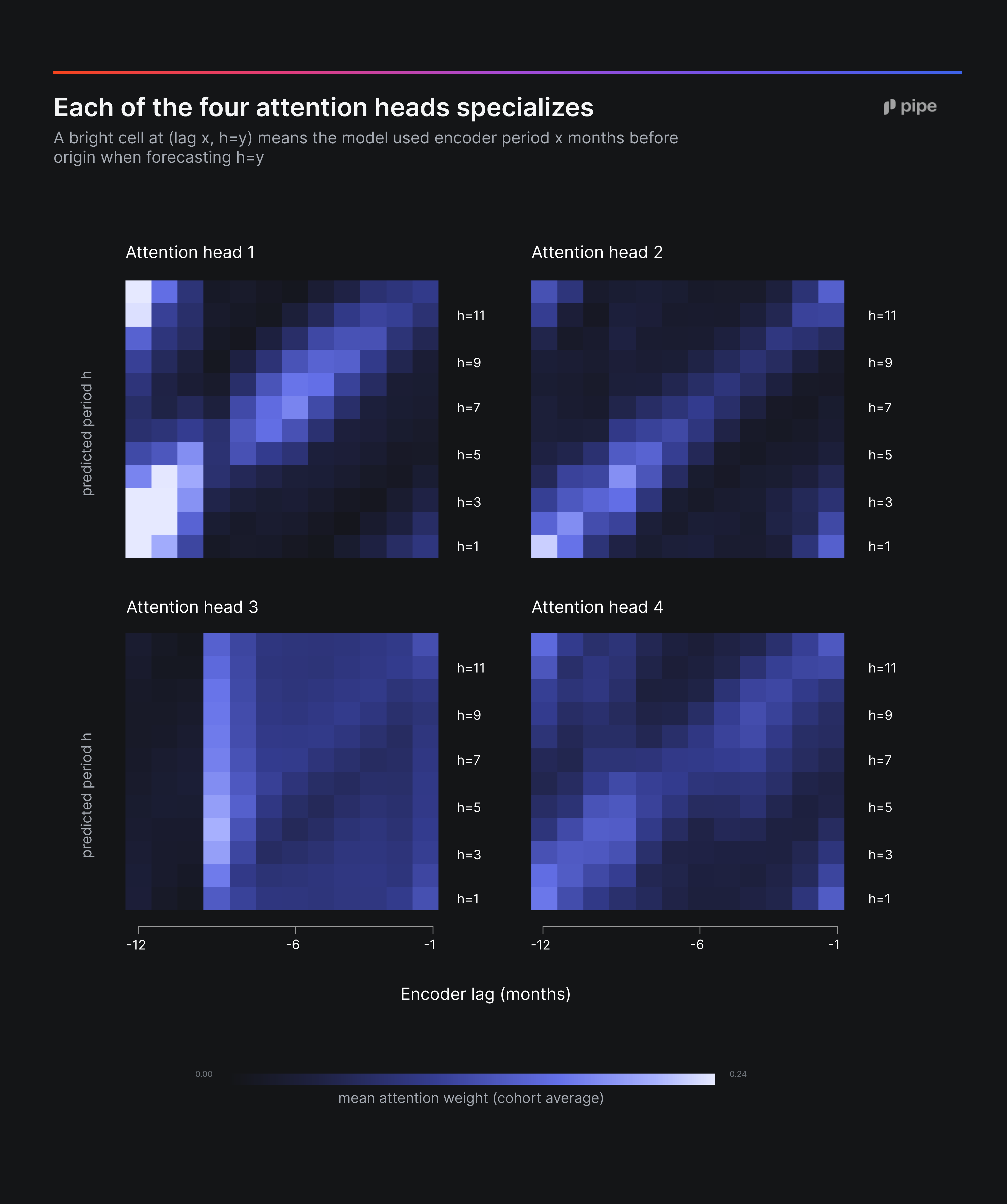Per-head attention, cohort mean

Figure 9: Cohort-mean attention weights for each of the four heads, averaged over 24,204 merchants. Each panel shows which past period (x-axis, encoder lag) the head leaned on when forecasting each future period (y-axis, horizon).

Per-archetype shifts. Decomposing the cohort by qualitative archetype (growing, declining, seasonal, stable, volatile, short history), attention patterns shift in interpretable ways. For merchants on a growing trajectory, the most recent observation receives approximately 4 percent of attention weight: the model leans on the longer arc. For merchants on a declining trajectory, the same recent observation receives approximately 15 percent: the model leans on recent evidence. The four-fold shift is learned from revenue sequences alone, with no trajectory label provided as input.

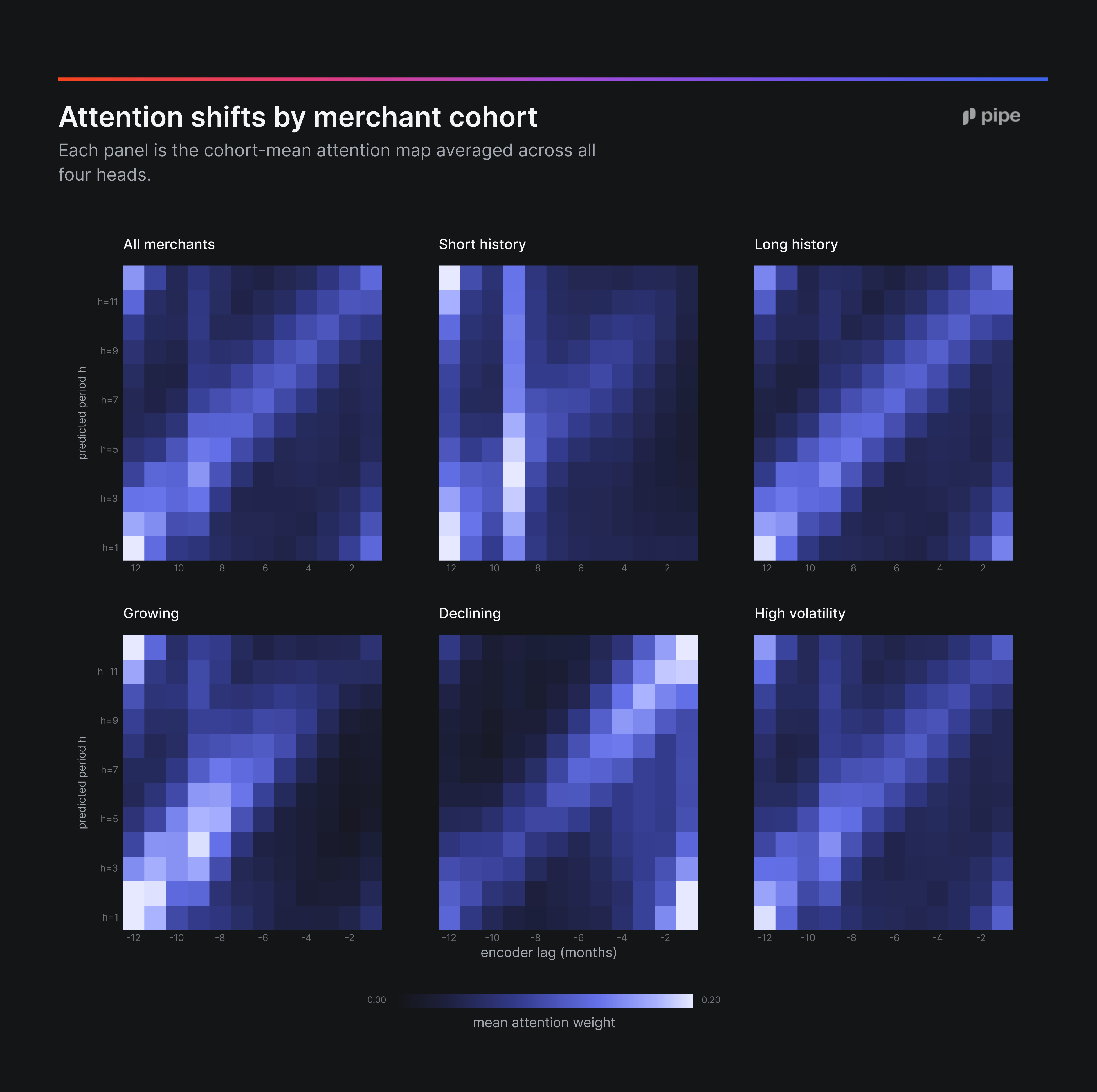Attention by merchant cohort

Figure 10: Attention patterns by merchant archetype, averaged over the four heads. The growing and declining panels show the contrast most clearly: declining merchants pull attention toward the recent end of the window, growing merchants toward the deep end.

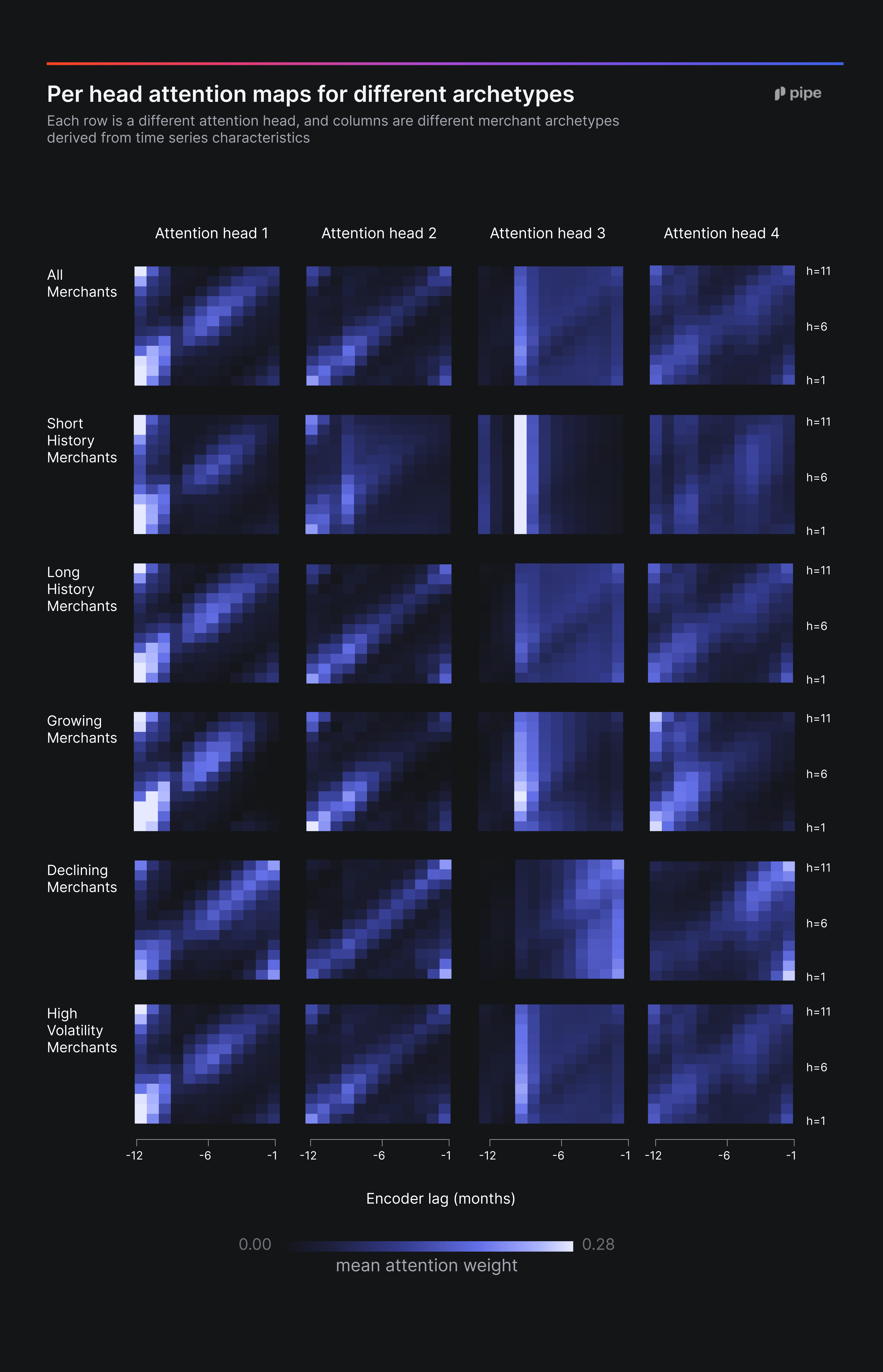Per-head, per-cohort decomposition

Figure 11: The four attention heads (rows) broken down across six merchant archetypes (columns). Reading across a row shows how a single head shifts its behavior between cohorts; reading down a column shows which heads carry the cohort-specific signal.

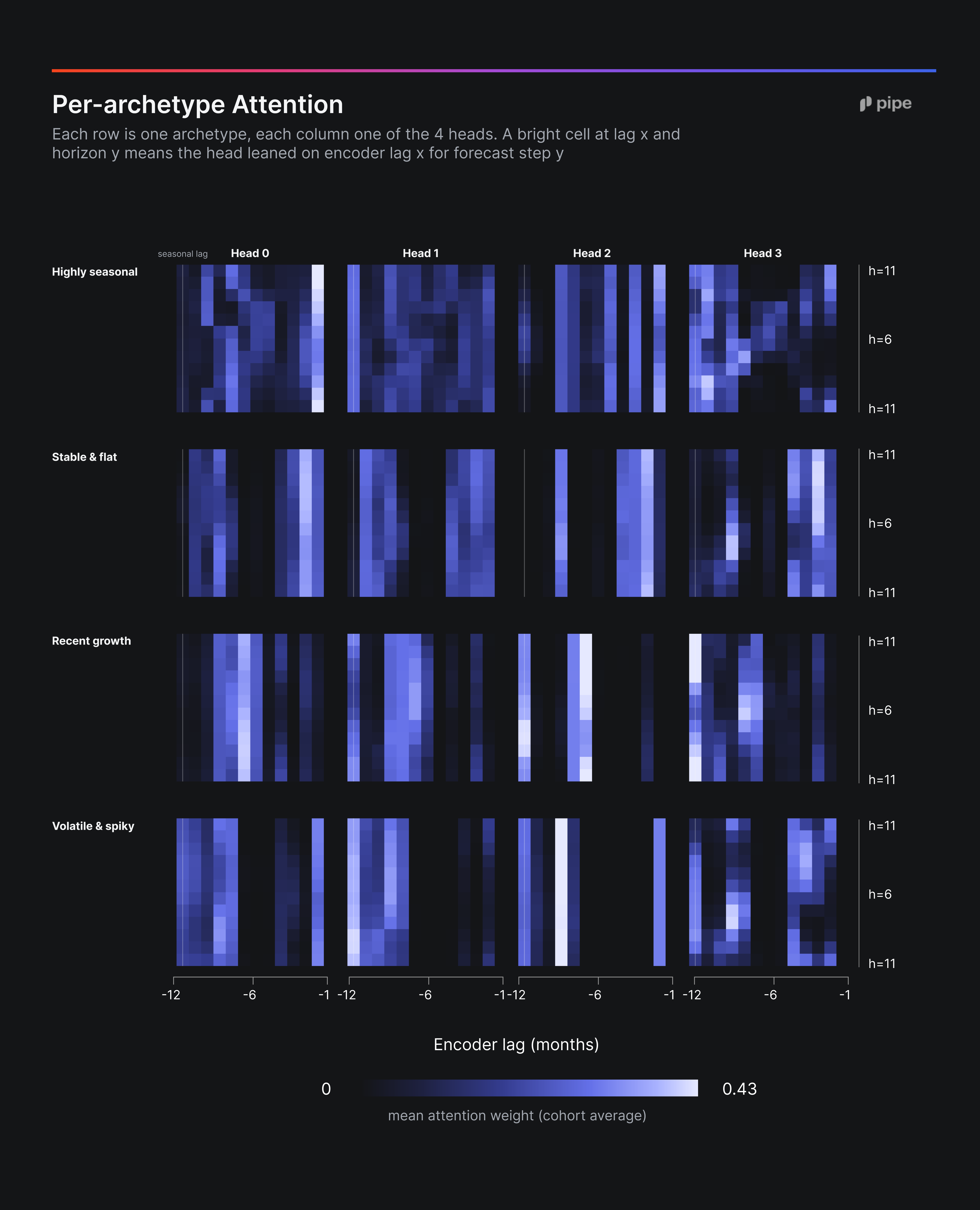Per-archetype attention, four exemplars

Figure 12: Each row is one merchant archetype; each column is one of the four attention heads. A bright cell at (encoder lag 𝑥, horizon ℎ) means the head leaned on encoder period 𝑥 when forecasting period ℎ. Maps are averaged across the four exemplar merchants per row from Figure 5.

Per-merchant entropy as a coverage diagnostic. The distribution of attention entropy across the cohort is bimodal. The bulk of merchants sit around normalized entropy 0.55 (a moderate anchor on one or two past periods). A long right tail above 0.85 corresponds almost entirely to merchants whose encoder window is zero-padded due to short platform history. The model is signaling, through the diffuseness of its own attention, where it lacks enough signal to anchor. This functions as a runtime coverage diagnostic for short-history merchants without requiring an auxiliary classifier.

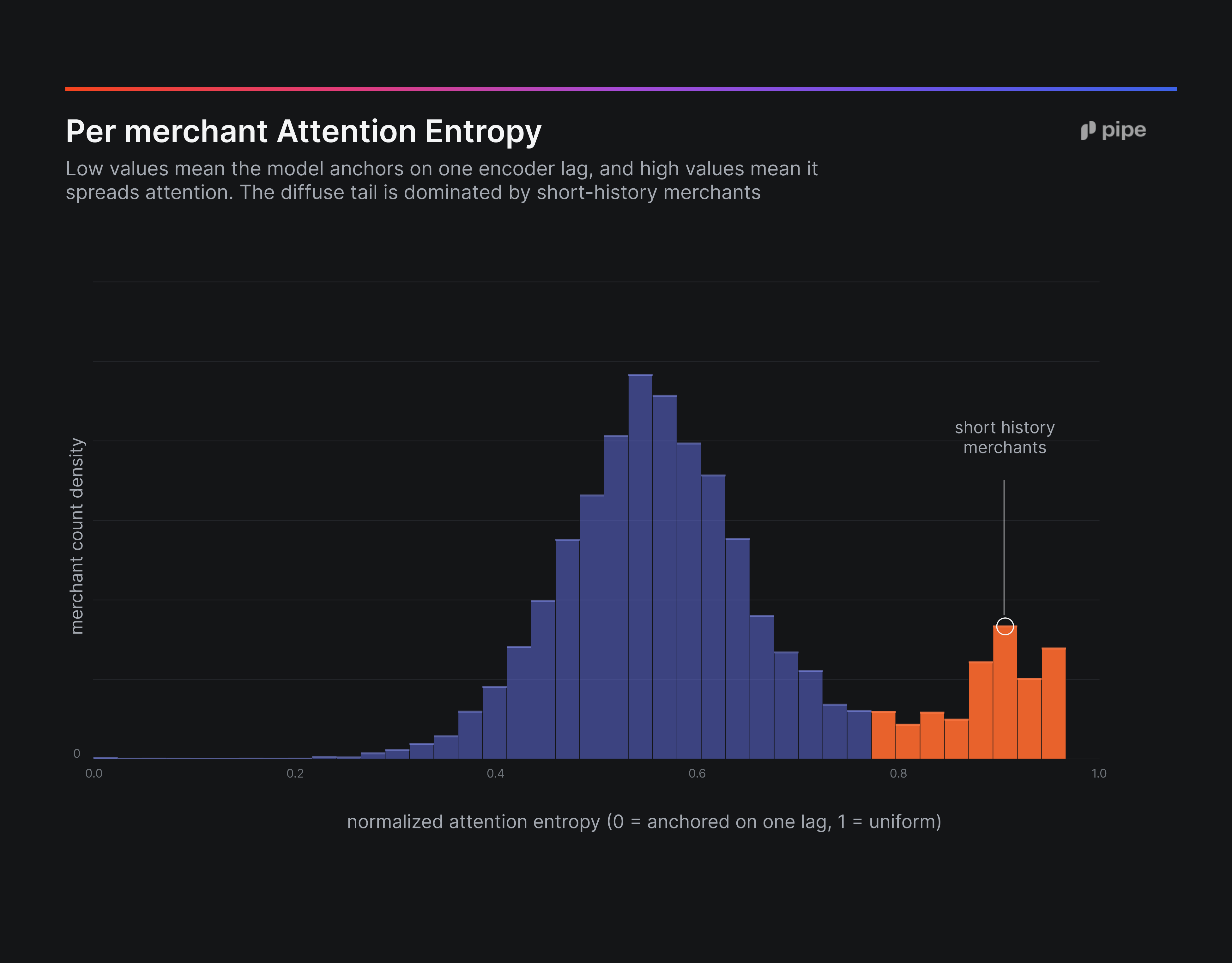Per-merchant attention entropy

Figure 13: Distribution of attention concentration across the 24,204 merchants. The bulk sit around 0.55 (a moderate anchor on one or two past periods); the long right tail above 0.85 corresponds almost entirely to short-history merchants where the model spreads attention evenly because there is little signal to anchor on.

9. Discussion

A year of production operation revised our prior on what mattered. Within the modern neural forecasting family, the architecture decision is close to a draw on this problem class against the classical ETS methods. The decisions that moved the neural models were the loss function, which shaped the credit posture; the choice to emit a distribution rather than a point, which created a richer policy surface; and the use of attention probes as runtime diagnostics rather than post-hoc explanations.

The most consequential empirical finding is that a forecaster trained on revenue alone produces an uncertainty signal — specifically the width of its lower tail — that is monotonically aligned with the deployed PD model. This does not require the forecaster to be retrained as a risk model, and it does not require additional labels. It is already present in the output of a calibrated distributional forecaster and is discarded by any system that consumes only the median. Whether the same signal stratifies realized friction at the merchant level is an open question; our simulator backtest did not produce a monotone reading there.

Limitations

Overfit risk on the rolling-origin protocol. As noted in §2, train and test windows are temporally disjoint, but merchants are not: a merchant with training observations through period T can have test observations at T+H, and we do not currently hold out a disjoint cohort of merchants the model has never seen at any prior point. The protocol controls temporal leakage but not merchant-identity recall through encoder patterns or idiosyncratic seasonality. Performance on truly new merchants, partner-two onboarding is the first such test, is the question this article does not answer.

Single-platform, single-regime. The training panel spans one partner's history during a benign macro period. Architecture, loss, and calibration findings are from that one cohort; we are watching whether they replicate on partner-two and partner-three. The distributional output is calibrated within the observed regime, we do not claim coverage on regime shifts or out-of-distribution events, and any forecaster of this class fits one epoch and must be re-evaluated past its boundaries. Production monitoring (calibration tracking, attention entropy, sub-1% leakage detection) is the only line of defense against silent degradation outside the training regime.

Simulator does not model the behavioral effect of credit. The 18-month backtest replays each merchant's actual revenue under a counterfactual policy. It does not model how receiving credit changes the merchant's revenue trajectory or operating decisions. The new policy will extend credit to merchants who did not previously receive any; the realized effect on those merchants is unmodeled and could go either way (capital-enabled growth, or overproduction in cases where staying unfunded would have been stable). A prospective rollout with random assignment among currently-undecisioned merchants is the only way to bound this, and it is the test we owe the next iteration of this work.

Short-history merchants. Fall below the encoder threshold; we currently route them to the classical baseline. Few-shot transfer and attention-aware sizing are the candidate next methods.

These are the analyses we expect to run next.

References

Challu, C., et al. (2023). NHITS: Neural hierarchical interpolation for time series forecasting. AAAI, 37(6), 6989–6997.

Chernozhukov, V., Fernández-Val, I., & Galichon, A. (2010). Quantile and probability curves without crossing. Econometrica, 78(3), 1093–1125.

Das, A., et al. (2023). Long-term forecasting with TiDE. arXiv:2304.08424.

Han, X., et al. (2024). Reversible mixture-of-KAN for time series forecasting. arXiv:2408.11306.

Hyndman, R. J., et al. (2008). Forecasting with exponential smoothing. Springer.

Lim, B., Arık, S. Ö., Loeff, N., & Pfister, T. (2021). Temporal fusion transformers for interpretable multi-horizon time series forecasting. International Journal of Forecasting, 37(4), 1748–1764.

Makridakis, S., Spiliotis, E., & Assimakopoulos, V. (2022). The M5 accuracy competition. International Journal of Forecasting, 38(4), 1346–1364.

Salinas, D., et al. (2020). DeepAR: Probabilistic forecasting with autoregressive recurrent networks. International Journal of Forecasting, 36(3), 1181–1191.

Makridakis, S., Spiliotis, E., & Assimakopoulos, V. (2022). The M5 accuracy competition. International Journal of Forecasting, 38(4), 1346–1364.

Montero-Manso, P., & Hyndman, R. J. (2021). Principles and algorithms for forecasting groups of time series: Locality and globality. International Journal of Forecasting, 37(4), 1632–1653.

Salinas, D., et al. (2020). DeepAR: Probabilistic forecasting with autoregressive recurrent networks. International Journal of Forecasting, 36(3), 1181–1191.

Vaswani, A., et al. (2017). Attention is all you need. NeurIPS 2017.

Wen, R., et al. (2017). A multi-horizon quantile recurrent forecaster. arXiv:1711.11053.

Zeng, A., et al. (2023). Are transformers effective for time series forecasting? AAAI, 37(9), 11121–11128.